Linear Tools Review - Part 1 - Complete Response From Diff Eq Description

Open access peer-reviewed chapter

Solution of Differential Equations with Applications to Engineering Issues

Submitted: May 6th, 2016 Reviewed: Jan 19th, 2017 Published: March 15th, 2017

DOI: 10.5772/67539

IntechOpen Downloads

6,698

Total Chapter Downloads on intechopen.com

Altmetric score

Overall attention for this chapters

Abstract

Over the final hundred years, many techniques have been developed for the solution of ordinary differential equations and partial differential equations. While quite a major portion of the techniques is merely useful for academic purposes, there are some which are of import in the solution of real problems arising from science and technology. In this chapter, only very limited techniques for solving ordinary differential and partial differential equations are discussed, every bit it is impossible to cover all the available techniques even in a volume form. The readers are then suggested to pursue farther studies on this issue if necessary. After that, the readers are introduced to two major numerical methods ordinarily used past the engineers for the solution of real engineering problems.

Keywords

• differential equations
• analytical solution
• numerical solution

• Cheng Yung Ming*

  • Department of Civil and Environmental Engineering science, Hong Kong Polytechnic University, Hong Kong SAR, Mainland china

*Address all correspondence to: ceymchen@polyu.edu.hk

1. Introduction

1.ane. Classification of ordinary and partial equations

To begin with, a differential equation can be classified as an ordinary or fractional differential equation which depends on whether only ordinary derivatives are involved or partial derivatives are involved. The differential equation can also exist classified equally linear or nonlinear. A differential equation is termed as linear if information technology exclusively involves linear terms (that is, terms to the ability i) of y, y ′, y ″ or higher society, and all the coefficients depend on only i variable x as shown in Eq. (1). In Eq. (i), if f ( x ) is 0, and so nosotros term this equation as homogeneous. The general solution of non-homogeneous ordinary differential equation (ODE) or partial differential equation (PDE) equals to the sum of the fundamental solution of the respective homogenous equation (i.e. with f ( 10 ) = 0) plus the particular solution of the non-homogeneous ODE or PDE. On the other hand, nonlinear differential equations involve nonlinear terms in any of y, y ′, y ″, or higher order term. A nonlinear differential equation is mostly more than difficult to solve than linear equations. Information technology is common that nonlinear equation is approximated as linear equation (over acceptable solution domain) for many practical problems, either in an analytical or numerical form. The nonlinear nature of the trouble is and so approximated as series of linear differential equation past simple increment or with correction/difference from the nonlinear behaviour. This approach is adopted for the solution of many non-linear engineering problems. Without such procedure, almost of the non-linear differential equations cannot be solved. Differential equation can further be classified by the club of differential. In full general, higher-order differential equations are hard to solve, and analytical solutions are not available for many higher differential equations. A linear differential equation is generally governed by an equation form equally Eq. (1).

d n y d x due north + a 1 ( x ) d northward − 1 y d x due north − 1 + … + a n ( x ) y = f ( x )

E1

"Non-linear" differential equation can mostly be further classified as

1. Truly nonlinear in the sense that F is nonlinear in the derivative terms.

   F ( x 1 , ten one , x due north , u , ∂ u ∂ 10 1 , ∂ u ∂ x 2 , ∂ 2 u ∂ x one ∂ 10 2 ) = 0

   E2

2. Quasi-linear 1st PDE if nonlinearity in F simply involves u but not its derivatives

   A 1 ( ten ane , ten 2 , u ) ∂ u ∂ x 1 + A 2 ( x 1 , x 2 , u ) ∂ u ∂ x 2 = B ( x 1 , x 2 , u )

   E3

3. Quasi-linear 2d PDE if nonlinearity in F only involves u and its first derivative but not its second-order derivatives

   A 11 ( x 1 , x 2 , u , ∂ u ∂ x ane , ∂ u ∂ ten 2 ) ∂ 2 u ∂ ten ane 2 + A 12 ( x 1 , x 2 , u , ∂ u ∂ ten 1 , ∂ u ∂ x 2 ) ∂ ii u ∂ x 1 ∂ x 2 + A 22 ( x 1 , x ii , u , ∂ u ∂ x 1 , ∂ u ∂ x 2 ) ∂ ii u ∂ x two two = F ( x 1 , x 2 , u ∂ u ∂ x i , ∂ u ∂ x 2 )

   E4

Examples of differential equations :

1. d y d x = 3 x + ii ; first-gild ODE (linear)/nonhomogeneous

2. ( y − 2 x ) d y − 3 y d ten = 0 ; first-order ODE (nonlinear)/homogenous

3. d two y d t two + t 2 y ( d y d t ) 3 + y = 0 ; second-guild ODE (nonlinear)/homogenous

4. d 4 x d t 4 + 5 d 2 x d t 2 + 7 x = south i due north t ; 4th-order ODE (linear)/nonhomogeneous

5. ∂ z ∂ ten + ∂ z ∂ y = 2 z ; commencement-order PDE (linear)/homogeneous

6. ∂ 2 u ∂ x ii + ∂ 2 u ∂ y 2 + 4 10 + 3 y − u z = 0 ; second-order PDE (linear)/nonhomogeneous

7. 10 ∂ 2 u ∂ ten 2 + 2 u ∂ 2 u ∂ y 2 + 3 u 2 = 0 ; second-order PDE (linear)/homogeneous

8. d u d x − d 5 d 10 = 6 x ; 1st ODE (linear) for ii unknowns/nonhomogeneous

1.ii. Typical differential equations in engineering problems

Many engineering bug are governed by different types of fractional differential equations, and some of the more than important types are given below.

1. Tricomi equation : y ∂ ii u ∂ x 2 + ∂ 2 u ∂ y 2 = 0 { y > 0 : e fifty fifty i p t i c y < 0 : h y p eastward r b o l i c

2. Laplace equation (or variants): ∂ 2 φ ∂ 10 2 + ∂ ii φ ∂ y ii = ∇ 2 φ = 0

3. Poisson's equation: ∂ 2 φ ∂ x 2 + ∂ 2 φ ∂ y two = f ( x , y )

4. Helmholtz equation: ∂ 2 φ ∂ x 2 + ∂ 2 φ ∂ y 2 + c 2 φ = 0

5. Plate bending: ∇ 2 ∇ 2 w = ∇ four due west = q D

6. Moving ridge equation (1D-3D) : ∂ 2 u ∂ t 2 − c 2 ( ∂ 2 u ∂ 10 2 + ∂ ii u ∂ y 2 ) = 0

7. Fourier equation: ∂ T ∂ t = α ( ∂ ii T ∂ x 2 )

There are many methods of solutions for dissimilar types of differential equations, but most of these methods are not commonly used for applied issues. In this chapter, the nearly important and bones methods for solving ordinary and partial differential equations volition be discussed, which will and so exist followed by numerical methods such every bit finite difference and finite element methods (FEMs). For other numerical methods such as boundary element method, they are less normally adopted past the engineers; hence, these methods volition not be discussed in this chapter.

1.3. Separable differential equations

For equations which can exist expressed in separable form every bit shown below, the solution tin can exist obtained hands equally

d y d x = F ( x , y ) d y Φ ( y ) = f ( ten ) d x ∫ ​ d y Φ ( y ) = ∫ ​ f ( x ) d ten + c

E5

Thou ( 10 , y ) d x + Northward ( x , y ) d y = 0 Chiliad ( x ) d x = − N ( y ) d y

E6

then ∫ ​ M ( x ) d ten = − ∫ ​ N ( y ) d y + c

E7

Example:

d y d x = 10 three ( y 2 + one ) ⇒ d y y two + one = ten three d x ∫ ​ d y y 2 + 1 = ∫ ​ x three d x + c ⇒ t a n − 1 y = i iv x iv + C ⇒ y = t a n ( ane 4 x 4 + c )

E9000

Instance:

d y d 10 = iii 10 2 + 4 x + 2 2 ( y − one ) subject to y ( 0 ) = − ane

Since this is a separable function, the problem can exist solved as

ii ( y − 1 ) d y = ( three x 2 + four x + two ) d x y 2 − 2 y = x iii + 2 x two + 2 x + c

E9008

Based on the boundary condition, c = 3, hence y 2 − 2 y = x 3 + 2 x ii + 2 10 + three .

This quadratic equation in y ² can be solved with two solutions past the quadratic equation as

y = ane − ten 3 + 2 x ii + ii 10 + four  and y = 1 + x iii + 2 x 2 + 2 x + 4 .

E9001

Since the 2d solution does non satisfy the boundary condition, it will not exist accustomed; hence, the solution to this differential equation is obtained.

ane.4. Variation of parameters

For the following equation form, it is possible to solve it past variations of parameters.

Put y = c ( x ) e ∫ ​ p ( x ) d x . Past differentiating, information technology gives d y d 10 = d c ( x ) d ten due east ∫ ​ p ( x ) d x + c ( x ) p ( ten ) e ∫ ​ p ( 10 ) d x ︸ p ( x ) y . Substitute it to the original ODE d c ( ten ) d 10 = Q ( 10 ) e − ∫ ​ p ( x ) d x . Comparing the terms, information technology gives

c ( x ) = ∫ ​ Q ( x ) eastward − ∫ ​ p ( x ) d ten d x + c ¯ .

E9

Example:

( x + 1 ) d y d x − n y = e x ( x + 1 ) due north + 1

E9003

This equation is now expressed as

d y d x = p ( x ) y + Q ( x ) d y d x = n 10 + ane y + eastward x ( ten + 1 ) n ︸ Q ( x )

E9002

For 10 ≠ −1

Solving the homogeneous office of the ODE

d y d x = northward x + one y then d y y = northward 10 + i d 10

l northward | y | = n l northward | x + 1 | + c 1 y = c ( x + 1 ) n

E9005

Wait for solution y = c ( ten ) ( x + one ) n , where c ( ten ) is the variation of parameters. Substitute it to the ODE

d c ( x ) d 10 ( 10 + ane ) n + due north c ( 10 ) ( x + 1 ) north − 1 = n c ( ten ) ( ten + 1 ) n − ane + due east x ( x + 1 ) north d y d x = north x + 1 y + e x ( 10 + ane ) n

E9006

Comparison gives d c ( x ) d x = east x

Integration of this equation gives c ( x ) = e x + C ¯

General solution is hence given past y = ( x + 1 ) northward ( eastward ten + C ¯ )

The Bernoulli equation is an important equation blazon which can exist solved in a similar way by variation of parameters. Consider the following course of equation

S t e p 2 :  So d z d x = ( ane − due north ) y − n d x d y d z d ten = ( 1 − northward ) P ( x ) z + ( 1 − n ) Q ( ten )

E12

The non-linear ODE at present becomes linear ODE. It tin can be solved past formula

Step 3: northward = −1, z = y ⁱⁱ. Inverting z to get y

z = e ∫ i x d x ( ∫ x 2 e − ∫ 1 x d x d x + c ) = c x + 1 ii x iii

E15

Back substitution of z = y ii

1.5. Homogeneous equations

For equation of the following type, where all the coefficients are constant, it can be evaluated according to different atmospheric condition.

d y d x = a ane x + b 1 y + c 1 a ii x + b 2 y + c 2

E17

Case 1: c ane = c 2 = 0

d y d 10 = a 1 ten + b 1 y a 2 x + b 2 y = a 1 + b 1 y x a 2 + b 2 y x = thousand ( y x )

E18

Step i: Prepare u = y x , then d y d x = x d u d ten + u

Step 2: d u d x = yard ( u ) − u ten . The resulting non-linear ODE is hence separable and tin can be solved implicitly.

Step three: Inverting u to go y .

Example 2: | a 1 a 2 b 1 b 2 | = 0

a one b 2 − a 2 b one = 0 then a 1 a 2 = b 1 b 2 = k

d y d x = a 1 10 + b 1 y + c 1 a 2 x + b 2 y + c 2 = chiliad ( a two ten + b 2 y ) + c 1 a 2 x + b 2 y + c ii = f ( a 2 10 + b 2 y )

E19

Past change of variables every bit u = a 2 x + b 2 y

d u d x = a ii + b 2 d y d x = a 2 + b two f ( u ) , and so

The resulting non-linear ODE is now separable and can be solved.

Case three: | a 1 a 2 b 1 b ii | ≠ 0 c 1 ≠ 0 and c 2 ≠ 0

Set up { a 1 x + b 1 y + c ane = 0 a ii x + b 2 y + c 2 = 0 . Intersecting bespeak of these ii lines on xy - aeroplane and (α, β) ≠ 0

x y − aeroplane and ( α , β ) ≠ ( 0 , 0 )

E21

Utilise change of variables

{ X = x − α Y = y − β { 10 = X + α y = Y + β

E22

a 1 x + b 1 y + c 1 = a 1 ( Ten + α ) + b 1 ( Y + β ) + c i = a 1 X + b i Y + ( a 1 α + b 1 β + c 1 ) a ii x + b 2 y + c 2 = a two ( X + α ) + b 2 ( Y + β ) + c 2 = a 2 Ten + b 2 Y + ( a 2 α + b 2 β + c 2 )

E23

The original ODE will now become d Y d 10 = a 1 X + b 1 Y a 2 X + b 2 Y which is homogeneous and separable!

Example: d y d x = ten + y − one x − y + 3

Solve for { ten + y − ane = 0 x − y + 3 = 0 we have α = − i , β = 2

Change of variables X = x + 1, Y = y − 2

So, d Y d X = d y d x = 10 + y − one x − y + 3 = 10 + Y X − Y = ane + Y X 1 − Y 10

Use a change of variable u = Y X 10 d u d X = 1 + u two 1 − u ( one − u ) d u i + u 2 = d 10 Ten

⇒ t a due north − i u − i 2 l due north ( 1 + u ii ) = l n | Ten | + c ⇒ t a north − 1 u = l n [ 1 + u 2 X ] + c = l north [ ( 10 2 + Y 2 ) ] + c ⇒ t a n − ane ( y − ii ten + 1 ) = l n ( x + 1 ) 2 + ( y − 2 ) ii + c

E9007

There are various tricks to solve the differential equations, like integration factors and other techniques. A very adept coverage has been given by Polyanin and Nazaikinskii [29] and will not be repeated here. The purpose of this department is just for illustration that various tricks take been developed for the solution of simple differential equations in homogeneous medium, that is, the coefficients are constants inside a continuous solution domain. The readers are as well suggested to read the works of Greenberg [14], Soare et al. [34], Nagle et al. [28], Polyanin et al. [xxx], Bronson and Costa [four], Holzner [eighteen], and many other published books. There are many elegant tricks that have been developed for the solution of unlike forms of differential equations, but simply very few techniques are actually used for the solution of existent life issues.

one.6. Partial differential equations

In many engineering or science problems, such as heat transfer, elasticity, quantum mechanics, water flow and others, the problems are governed by partial differential equations. By nature, this type of trouble is much more than complicated than the previous ordinary differential equations. There are several major methods for the solution of PDE, including separation of variables, method of characteristic, integral transform, superposition principle, modify of variables, Lie group method, semianalytical methods equally well every bit various numerical methods. Although the existence and uniqueness of solutions for ordinary differential equation is well established with the Picard-Lindelöf theorem, only that is not the example for many fractional differential equations. In fact, analytical solutions are not bachelor for many partial differential equations, which is a well-known fact, peculiarly when the solution domain is nonregular or homogeneous, or the material properties change with the solution steps.

1.half dozen.1. Classification of 2d-order PDE

Refer to the following general 2d-order fractional differential equation:

A ∂ ii u ∂ 10 2 + B ∂ 2 u ∂ x ∂ y + C ∂ 2 u ∂ y 2 + D ∂ u ∂ 10 + E ∂ u ∂ y + F u + G = 0

E24

To begin with, let us consider a review of conic curves (ellipse, parabola and hyperbola)

The conic bend can be classified with the following criterion.

B 2 − 4 A C = { > 0 hyperbola = 0 parabola < 0 ellipse

E26

Following the conic curves, the general partial differential is likewise classified according to similar criterion as

Classification { B 2 − 4 A C > 0 : elliptic B 2 − iv A C = 0 : parabolic B 2 − 4 A C < 0 : hyperbolic

E27

This classification was proposed past Du Bois-Reymond [41] in 1839. In this department, only some of the more common techniques are discussed, and the readers are suggested to read the works of Hillen et al. [16], Salsa [33], Polyanin and Zaitsev [31], Bertanz [ii], Haberman [xv] and many other published texts.

1.7. Parabolic type: estrus conduction/soil consolidation/diffuse equation

The post-obit equation form is commonly found in many applied science applications.

α 2 ∂ two u ∂ x 2 = ∂ u ∂ t , 0 < x < L , t > o

E28

Initial status: u ( ten , 0 ) = f ( x ) , 0 ≤ x ≤ 50

Boundary condition: u ( 0 , t ) = 0 , u ( L , t ) = 0 , t > 0

α ² is a abiding known as the thermal diffusivity or coefficient of consolidation. For soil consolidation trouble, the governing conditions are given by

Initial excess pore pressure

u eastward ( z , 0 ) = u i ( z ) , 0 ≤ z ≤ 2 d u east ( 0 , t ) = 0 , u eastward ( two d , t ) = 0 , t > 0

E29

Tuckered boundary

α 2 u x x = u t , 0 < ten < Fifty , t > 0 u ( 0 , t ) = 0 , u ( L , t ) = 0 , t > 0 u ( x , 0 ) = f ( x ) , 0 ≤ x ≤ L

E30

Assuming variable u ( x, t ) tin can be separated, using separation of variables

α 2 Ten ″ T = X T ′ X ″ X = 1 α two T ′ T X ″ X = ane α 2 T ′ T = − λ → { 10 ″ + λ X = 0 T ′ + α 2 λ T = 0

E32

A PDE now becomes ii ODE which can exist solved readily. Based on the boundary condition u ( 0 , t ) = 0 , u ( L , t ) = 0 , t > 0

u ( 0 , t ) = 10 ( 0 ) , T ( t ) = 0 Ten ( 0 ) = 0 , X ( 50 ) = 0 X ″ + λ 10 = 0 , Ten ( 0 ) = 0 , X ( L ) = 0

E33

This is an eigenvalue problem which has solution just for certain λ . The eigenvalues are given past

Hence the eigenfunctions are expressed as

X n ( x ) = s i northward ( n π x Fifty ) , n = 1 , ii , 3 …

E35

For the fourth dimension-dependent function T ,

d T T = − α two λ d t l n | T | = − α 2 n ii π ii t 50 2 + C

E37

hence T n = k n east − ( n π α / L ) two t , one thousand due north constant. The fundamental solutions are so expressed every bit

u ( ten , t ) = e − ( northward π α / L ) 2 t due south i n ( n π x L ) , n = ane , two , 3 …

E38

The Fourier series expansion in 10 is given by

u ( x , t ) = ∑ n = 1 ∞ c n u n ( x , t ) = ∑ n = i ∞ c n e − ( north π α / Fifty ) 2 t s i due north ( northward π x L )

E40

Initial condition is given every bit

u ( ten , 0 ) = f ( x ) = ∑ n = 1 ∞ c n s i n ( n π x 50 )

E41

∫ 0 L f ( 10 ) s i n ( chiliad π 10 L ) d ten = ∑ n = 1 ∞ c due north ∫ 0 L s i n ( thou π x 50 ) s i n ( n π x Fifty ) d ten ∫ 0 L f ( x ) south i due north ( n π ten 50 ) d 10 = c north ∫ 0 L s i n 2 ( m π x Fifty ) d x = c n 50 2

E8000

Solution of the soil consolidation equation is hence given past

u ( x , t ) = ∑ northward = 1 ∞ c n due east − ( n π α / L ) 2 t s i northward ( n π x L )

E42

c n = ii L ∫ 0 L f ( x ) s i n ( n π ten Fifty ) d x ( EulerFourier formulas )

E43

one.eight. I-dimensional wave equation

One-dimensional (1D) wave equation appears in many physical and engineering problems. For example, a vibrating string or pile driving procedure is given by this type of differential equation. This problem is besides commonly solved by the method of separation of variables

a 2 u x x = u t t , 0 < x < L , t > 0 u ( 0 , t ) = 0 , u ( L , t ) = 0 , t ≥ 0 u ( x , 0 ) = f ( x ) , u ( x , 0 ) = 0 , 0 ≤ x ≤ L

E44

Consider u ( 10, t ) is given by X ( x ) T ( t ). The moving ridge equation will requite

X ″ X = 1 a 2 T ′ T = − λ → { X ″ + λ x = 0 T ′ + a 2 λ t = 0

E45

The fractional differential equation will then be given by ii equivalent ODEs.

u t ( ten , 0 ) = Ten ( x ) T ' ( 0 ) = 0 , 0 ≤ ten ≤ L → T ' ( 0 ) = 0 u ( 0 , t ) = 10 ( 0 ) T ( t ) = 0 , u ( L , t ) = Ten ( L ) T ( t ) 0 ≤ x ≤ Fifty → T ' ( 0 ) = 0

E46

10 n ( x ) = s i northward ( northward π ten 50 ) , due north = 1 , two , 3 , …

E48

For the time-dependent part T ,

T ' ( 0 ) = 0 λ n = northward π / Fifty Then T ( t ) = k 1 c o due south ( north π a t / Fifty ) − thousand ii s i due north ( due north π a t / Fifty )

E51

Since T ' ( 0 ) = 0 yard 2 = 0

Therefore, T ( t ) = k 1 c o s ( n π a t / 50 )

Fundamental solution is given past

u n ( 10 , t ) = south i north ( n π 10 Fifty ) c o s ( n π a t 50 ) , n = 1 , 2 , 3 …

E52

The general solution is and so given by

u ( 10 , t ) = ∑ n = 1 ∞ c n u n ( ten , t ) = ∑ n = i ∞ c due north s i northward ( due north π x L ) c o due south ( n π a t 50 )

E53

Applying the boundary condition

u ( x , 0 ) = f ( x ) , 0 ≤ x ≤ L u ( x , 0 ) = f ( x ) = ∑ n = i ∞ c n s i n ( due north π 10 Fifty ) → c n = 2 Fifty ∫ 0 L f ( 10 ) s i north ( northward π x L ) d 10

E54

The last solution is then given past

u ( x , t ) = ∑ northward = one ∞ c n due south i n ( north π x L ) c o southward ( due north π a t 50 )

E55

c northward = ii Fifty ∫ 0 L f ( x ) s i due north ( due north π ten Fifty ) d x

E56

1.9. Laplace equation

Laplace equation forms an important governing condition for many types of problems. Some of the more than common forms are given by

1. three-dimensional Laplace equation u x x + u y y + u z z = 0

2. 2-dimensional heat conduction α two ( u x x + u y y ) = u t

3. ii-dimensional seepage problem ( thousand 10 u x ten + thou y u y y ) = 0

There are two major types of boundary weather condition to this problem:

1. Dirichlet problem: boundary conditions prescribed as u

2. Neumann problem: normal derivative u ₁₀ or u _y are usually prescribed on the boundary for many mathematical problems. This case can exist solved by the use of complex assay or series method for which many analytical solutions are available in the literature. In many anisotropic seepage bug, however, the normal of a derived quantity at any arbitrary direction (seepage menses normal to an impermeable surface) is 0 instead of u _ten or u _y being zero. For such cases, it is very hard to obtain the belittling solution if the solution domain is nonhomogeneous, and the use of numerical method such equally the finite element method appears to exist indispensable.

Consider the given Laplace equation, using separation of variables for the analysis.

u x ten + u y y = 0 , 0 < 10 < a , 0 < y < b u ( x , 0 ) = 0 , u ( 10 , b ) = 0 , 0 < x < a u ( 0 , y ) = 0 , u ( a , y ) = f ( y ) , 0 < y ≤ b

E57

Using separation of variables, u ( x , t ) = X ( x ) Y ( y )

X ″ Y + 10 Y ″ = 0 X ″ X = − Y ″ Y = λ → X ″ − λ X = 0 Y ′ + λ Y = 0

E58

u ( x , 0 ) = 0 , u ( ten , b ) = 0 , 0 < x < a u ( 0 , y ) = 0 , u ( a , y ) = f ( y ) , 0 < y ≤ b

E60

u ( 0 , y ) = X ( 0 ) Y ( y ) = 0 , 0 < y < b → X ( 0 ) = 0 , u ( x , 0 ) = X ( ten ) Y ( 0 ) = 0 , 0 < x < a → Y ( 0 ) = 0 , u ( x , b ) = X ( x ) Y ( b ) = 0 , 0 < x < a → Y ( b ) = 0 ,

E61

X ″ − λ Ten = 0 , X ( 0 ) = 0 Y ″ + λ Y = 0 , Y ( 0 ) = 0 , Y ( b ) = 0

E62

λ n = n two π 2 b two , Y due north ( y ) = s i n ( n π y b ) , due north = one , two , 3 , …

E63

X ″ − λ 10 = 0 , hence 10 ( x ) = k 1 c o southward h ( n π x / b ) − k two southward i n ( n π x / b )

Since 10 (0) = 0, k _i = 0

u n ( x , y ) = s i n h ( north π x b ) s i n ( due north π y b ) n = 1 , 2 , three …

E65

u ( a , y ) = f ( y ) , 0 ≤ y ≤ b u ( ten , y ) = ∑ n = 1 ∞ c n u n ( x , y ) = ∑ northward = i ∞ c n southward i n ( n π x b ) c o s ( n π y b )

E66

Based on the Fourier expansion every bit given by

∫ 0 b f ( y ) s i n ( m π y b ) d y = ∑ due north = 1 ∞ c n s i due north h ( n π a b ) ∫ 0 b s i n ( one thousand π y b ) s i due north ( n π y b ) d y ∫ 0 b f ( x ) southward i northward ( n π x b ) d 10 = s i northward h k π a b c n ∫ 0 b s i due north 2 ( n π x b ) d x = due south i northward h chiliad π a b c due north b 2 u ( a , y ) = f ( y ) = ∑ due north = ane ∞ c n s i n h ( n π a b ) due south i northward ( n π y b )

E67

c due north s i northward h ( n π a b ) = 2 b ∫ 0 b f ( y ) s i north ( n π y b ) d y c northward = 2 b s i n h ( due north π a b ) − ane ∫ 0 b f ( y ) s i n ( n π y b ) d y

E9009

1.10. Introduction to numerical methods

In general, analytical solutions are not available for most of the practical differential equations, every bit regular solution domain and homogeneous conditions may non be nowadays for practical bug. Moreover, the solution domain may exist indeterminate (free surface seepage flow), the displacement is big so that the solution may deform under move, or in an extreme example part of the fabric may tear off from the master body with continuous germination and removal of contacts. Many technology problems autumn into such category by nature, and the use of numerical methods volition exist necessary. Currently, there are several major numerical methods normally used by the engineers: finite difference method, finite element method, boundary element method and singled-out element. In that location are too other less common numerical methods bachelor for applied problems, and many researchers too effort to combine two or even more key numerical methods so every bit to achieve greater efficiency in the analysis. In full general, the solution domain is discretized into series of subdomains with many degrees of freedom. The number of variables or degrees of freedom may even exceed millions for large-scale problems, and sometimes very special textile properties are encountered so that the system is highly sensitive to the method of discretization and the method of solution. Similar to the ODE and PDE, information technology is incommunicable to hash out the details of all the numerical methods and the author choose to discuss the finite element method due to the wide acceptance of the method and this method is more suitable for general complicated methods.

Except for some simple bug with regular geometry and loading, it is very difficult to solve most of the boundary value problems with the yield of analytical solutions. Towards this, the use of numerical method seems indispensable, and the finite element is ane of the almost popular methods used past the engineers [32, 38]. In that location are two primal approaches to FEM, which are the weighted rest method (WRM) and variational principle, simply at that place are besides other less popular principles which may be more constructive under certain special cases. In finite element analysis of an elastic problem, solution is obtained from the weak form of the equivalent integration for the differential equations by WRM equally an approximation. Alternatively, different gauge approaches (due east.g. collocation method, least square method and Galerkin method) for solving differential equations tin can be obtained by choosing different weights based on the WRM and the Galerkin method appears to be the nigh pop approach in general.

Specifically, in elasticity for example, the principle of virtual piece of work (including both principle of virtual displacement and virtual stress) is considered to be the weak form of the equivalent integration for the governing equilibrium equations. Furthermore, the same weak grade of equivalent integration on the basis of the Galerkin method can also be evolved to a variation of a functional if the differential equations have some specific properties such as linearity and selfadjointness. Principles of minimum potential energy and complementary energy are two variational approaches equivalent to the fundamental equations of elasticity.

Since displacement is usually the basic unknown quantity in FEM, merely the principle of virtual deportation and minimum potential energy will be introduced in the following section. In this case, the FEM introduced herein is besides called displacement finite element method (DFEM). There are other ways to grade the footing of FEM with advantages in some cases, but these approaches are less general and volition non be discussed hither.

one.11. Principle of virtual displacement

The principle of virtual displacement is the weak form of the equivalent integration for equilibrium equations and force boundary weather. Given the equilibrium equations and force boundary weather condition in index notation,

σ i j , j + f i = 0 , ( in domain 5 )

E68

σ i j n j − T i = 0 , ( on domain boundary S σ )

E69

In WRM, without loss of generality, the variation of true displacement δ u i and its boundary value (i.east. − δ u i ) can be selected every bit the weight functions in the equivalent integration

∫ V δ u i ( σ i j , j + f i ) d 5 − ∫ Due south σ δ u i ( σ i j n j − T i ) d S = 0

E70

The weak form of Eq. (70) is given as

∫ V ( − δ ε i j σ i j + δ u i f i ) d V + ∫ S σ δ u i T i d South = 0

E71

It tin be seen clearly from Eq. (71) that the first item in the volume integral indicates the work washed by the stresses under the virtual strain (i.e. internal virtual work), while the remaining items point the piece of work washed by the body force and surface strength under the virtual displacement (i.e. external virtual piece of work). In other words, the summation of the internal and external virtual works is equal to 0, which is called the principle of virtual displacement. Under this case, nosotros can conclude that a force system volition satisfy the equilibrium equations if the summation of the work done by it nether any virtual displacement and strain is equal to 0.

one.12. Principle of minimum potential energy (PMPE)

Based on Eq. (71), we can deduce that

∫ V ( δ ε i j D i j k l ε chiliad l − δ u i f i ) d V + ∫ S σ δ u i T i d S = 0

E72

Due to the symmetry of the constitutive matrix D i j thou fifty , we can further obtain

( δ ε i j ) D i j k l ε thousand l = δ ( ane two D i j chiliad l ε i j ε k l ) = δ U ( ε one thousand n )

E73

where U ( ε m due north ) is the unit volume strain energy. Given the assumptions in linear elasticity

− δ ϕ ( u i ) = f i δ u i , − δ ψ ( u i ) = T i δ u i

E74

Eq. (72) is further simplified to

Π P is the total potential energy of the organisation, which is equal to the summation of the potential free energy of deformation and external force and can be expressed every bit

Π P = Π P ( u i ) = ∫ 5 ( ane 2 D i j grand l ε i j ε 1000 50 − f i u i ) d Five − ∫ Due south σ T i u i d S

E76

Eq. (75) shows that, among all the potential displacements, the total potential energy of system will have stationary value at the existent displacement, and it can be further verified that this stationary value is exactly the minimum value which is the principle of minimum potential energy.

1.13. General expressions and implementation procedure of FEM

The solution of a general continuum trouble by FEM ever follows an orderly step-by-step procedure which is piece of cake to be programmed and used by the engineers. For illustration, a three-node triangular element for plane problems is taken as an example to illustrate the general expressions and implementation procedures of FEM.

1.thirteen.1. Discretization of domain

The first step in the finite element method is to split the structure or solution region into subdivisions or elements. Hence, the structure is to be modelled with suitable finite elements. In general, the number, type, size, and organization of the elements are critical towards expert performance of the numerical analysis. A typical discretization with three-node triangular chemical element is shown schematically in Figure 1 .

Effigy 1.

Discretization of a two-dimensional domain with three-node triangular element.

Mesh generation tin can be a difficult procedure for a full general irregular domain. If only triangular element is to exist generated, this is a relatively simple work, and many commercial programs tin can perform well in this respect. There are besides some public domain codes (EasyMesh or Triangle written in C) which are sufficient for normal purposes. For quadrilateral or college elements, mesh generation is non that simple, and it is preferable to rely on the apply of commercial programs for such purposes.

1.xiii.2. Interpolation or displacement model

As can be seen from Figure one(b) , the nodal number of a typical three-node triangular element is coded in anticlockwise order (i.e. in the order of i, j and m ), and each node has two degrees of freedom (DOFs) or ii displacement components which is stored in a column vector in alphabetize note as follows:

Totally, each element has six nodal displacements, i.eastward. six DOFs. Putting all the displacements in a cavalcade vector, we can obtain the chemical element nodal deportation column matrix as

a e = [ a i a j a one thousand ] = [ u i v i u j v j u m v m ] T

E78

In FEM, a nodal displacement is chosen as the basic unknowns, and so interpolation at any arbitrary point is based on the three nodal displacements of each element, which is chosen a displacement way. For a 3-node triangular element, linear polynomial is utilized, and the element displacement in both ten -direction and y -direction are

Obviously, displacements of all the three nodes should satisfy Eqs. (79) and (80). By substituting the six nodal displacement components into these equations, it is piece of cake to obtain another form of displacement mode equally

where

N i = one two A ( a i + b i ten + c i y ) ( i , j , k ) .

E83

In Eq. (81), Due north i , North j and N m denote the interpolation part or shape function for the 3 nodes, respectively. A is the expanse of the chemical element, and a i , b i , c i ⋯ , c m are constants related to the coordinates of the iii nodes. Similarly, Eqs. (81) and (82) can also be expressed in the grade of matrix as

u = [ u v ] = [ N i 0 N j 0 N thousand 0 0 N i 0 N j 0 N m ] [ u i five i u j v j u one thousand v thou ] = Northward a e

E84

where North is the shape function matrix and a e is the chemical element nodal deportation vector. For the geometric equations, element strains are

ε = [ ε 10 ε y γ ten y ] = 50 u = L Northward a eastward = Fifty [ N i N j N yard ] a e = [ B i B j B yard ] a due east = B a e

E85

where Fifty is the differential operator and B is the element strain displacement matrix which tin can be given as

B i = L N i = [ ∂ ∂ x 0 0 ∂ ∂ y ∂ ∂ y ∂ ∂ x ] [ N i 0 0 Due north i ] = [ ∂ Due north i ∂ x 0 0 ∂ N i ∂ y ∂ North i ∂ y ∂ N i ∂ x ] ( i , j , grand )

E86

Substitute Eq. (85) by the stress-strain relation,

σ = [ σ ten σ y τ x y ] = D ε = D B a e = Due south a e

E87

where

S = D B = D [ B i B j B 1000 ] = [ S i S j Southward 1000 ]

E88

S is chosen the element stress matrix. It should be noted that both the strain and stress matrices are constant for each element, because in a three-node triangular element, the deportation mode is a commencement-order function, and differentiating this role volition give a abiding part.

one.13.3. Stiffness equilibrium equation (SEE) of FEM derived from PMPE

For rubberband plane issues, the total potential energy Π P in Eq. (76) can be expressed in matrix formulation every bit follows:

∏ P = ∫ Ω ane two ε T D ε t d 10 d y − ∫ Ω u T f t d x d y − ∫ S σ u T T t d S

E89

where t, f , and T denote the thickness, body force and surface force, respectively. For an FEM problem, the total potential free energy is the summation of that from all the elements. Therefore, substituting Eqs. (84) and (85) into Eq. (89) gives

Π P = ∑ e Π P e = ∑ e ( a e T ∫ Ω e 1 ii B T D B t d ten d y a due east ) − ∑ e ( a e T ∫ Ω due east N T f t d 10 d y ) − ∑ eastward ( a e T ∫ S σ e Northward T T t d x d y )

E90

Eq. (ninety) can be viewed every bit

K e = ∫ Ω due east B T D B t d x d y , P f e = ∫ Ω east Due north T f t d x d y P Due south e = ∫ S σ east N T T t d x d y , P due east = P f e + P S e

E91

where Yard e and P due east are named as the element stiffness matrix and equivalent element nodal load matrix, respectively. Substitute Eq. (91) to Eq. (xc), the total potential energy of the construction can be simplified as

Π P = a T 1 2 ∑ e ( K due east ) a − a T ∑ due east ( P east )

E92

Given

Eq. (92) is further simplified as

where One thousand and P are global stiffness matrix and global nodal load matrix, respectively.

For PMPE, the variation of Π P is equal to 0 and the unknown variable is a , thus Eq. (75) gives

which finally comes to the Run across of FEM as

From Eq. (93), nosotros know that the global stiffness matrix and the global load matrix are the aggregation of the chemical element stiffness matrices and equivalent element nodal load matrices, respectively. Specifically, in lodge to solve Eq. (93), element stiffness matrix, element equivalent nodal load vector, global stiffness matrices and global nodal load vector are all determined together with some given displacement boundary conditions. Without the provision of adequate boundary condition, the system is atypical as rigid body movement will produce no stress in the system and such mode will be nowadays in the SEE.

i.13.iv. Derivation of element stiffness matrices (ESM)

For a 3-node triangular element, the element strain matrix B is abiding, thus Eq. (91) gives

K due east = B T D B t A = [ Thousand i i K i j K i g K j i K j j K j m K m i M one thousand j K m yard ]

E96

of which the submatrix

K i j = [ k i j x x g i j x y k i j y x one thousand i j y y ]

E97

K i j indicates the i th nodal force along the x- and y -directions in the Cartesian coordinate system when the displacement of the j th node is unit of measurement along the x- and y -directions, which can be easily obtained. Moreover, the chemical element stiffness matrix is symmetric, and the computational memory required in an FEM program can be reduced by using this property.

Information technology should be noted that for a higher gild triangular chemical element (e.thou. half-dozen-node triangular element) or quadrilateral chemical element for which higher lodge terms are involved, the strain matrix B is non constant whatsoever more so that the element stiffness matrix needs to be evaluated by numerical integration (direct integration is seldom adopted). Towards this, numerical integration methods such as the Gaussian integration or the Newton-Cotes integration can exist utilized.

one.thirteen.5. Assembling of ESMs and ENLMs

For an FEM procedure, we need to solve Eq. (95) which is the global equilibrium equation. Most of the elements in the matrix Chiliad are 0 just because each node is only shared by a few surrounding elements. In view of that, a rectangular matrix can correspond the global stiffness matrix (which is a square matrix), and the half bandwidth D tin can be defined every bit

where NDIF denotes the largest absolute divergence between the element node numbers among all the elements in the finite element mesh.

In conclusion, the backdrop of the global stiffness matrix can exist summarized as: symmetric, banded distribution, singularity and sparsity. Among all the properties, singularity volition vanish by introducing appropriate boundary conditions to Eq. (95) to eliminate the rigid body motion. As well, other properties like banded distribution should be fully taken into consideration to reduce the computational memory and heighten the computation efficiency.

1.13.vi. Isoparametric element and numerical integration

Nearly of the engineering construction is not regular in shape, and some of them fifty-fifty have very complicated purlieus shapes. Although the use of triangular element tin can always fit a complicated boundary, the accuracy of this element is depression in full general. To cope with the irregular purlieus shape with a higher accurateness in analysis, i of the nearly common approaches is the utilize of higher-order element, and the isoparametric formulation is the most commonly used at nowadays. Consider an arbitrary four-node quadrilateral element as an example which is schematically shown in Figure 2 . If we tin find the transformation from Effigy 2(a) to (b), then it will become easier to behave numerical integration with complicated shapes for an capricious element. In Figure two(a), we define the Cartesian coordinate organization, while in Effigy ii(b) , we ascertain the local coordinate system (or natural coordinate system) inside a specific domain (i.e. ξ , η ∈ ( − 1 , 1 ) ). The relation between these ii kinds of coordinate organization tin exist described as

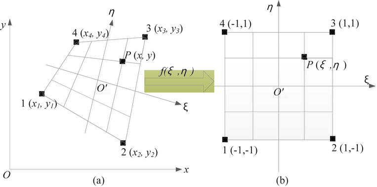
Figure 2.

Isoparametric transition.

which can be farther modified past the interpolation function at nodes in the local coordinate organization as follows:

ten = Σ i = 1 1000 N i ' x i , y = ∑ i = i m N ′ i y i

E100

where ( 10 i , y i ) are coordinates in the Cartesian coordinate arrangement corresponding to the i th node in local coordinate system, N i ' is interpolation part of the i th node in local coordinate system and m is the number of nodes called to transform the coordinates. Therefore, the regular element in the natural coordinate system can be transformed to the irregular element in the Cartesian coordinate system. The former element is chosen the parent element, while the latter is called the subelement. Specifically, Eq. (101) tin be further expanded as

{ 10 y } = [ N 1 0 N 2 0 N 3 0 N 4 0 0 N 1 0 Northward 2 0 Due north three 0 N iv ] { x 1 y 1 x 2 y 2 x 3 y 3 ten iv y 4 }

E101

Using the same interpolation functions, the element displacement model can be written as

{ u v } = [ Due north 1 0 N 2 0 N three 0 North four 0 0 Northward one 0 N two 0 N 3 0 N four ] { u 1 v 1 u 2 v two u three v 3 u 4 five iv }

E102

where J denotes the Jacobi matrix while the interpolation functions are given by

North 1 = 1 iv ( 1 + ξ ) ( 1 + η ) , Due north 2 = 1 4 ( ane − ξ ) ( one + η ) N 3 = 1 four ( 1 + ξ ) ( ane + η ) , N 2 = one 4 ( 1 − ξ ) ( 1 + η )

E103

As mentioned before, during the derivation of the element stiffness matrix and the equivalent load vector, the derivative of the shape function and the integration in element surface or volume in the Cartesian coordinate system are required. Since the shape functions adopted herein are expressed in natural coordinates, therefore, derivative and integration transformation relationships are essential when isoparametric chemical element is used.

i.13.7. Derivative and integral transformation

According to the police of partial differential,

∂ N i ∂ ξ = ∂ N i ∂ x ∂ ten ∂ ξ + ∂ Northward i ∂ y ∂ y ∂ ξ , ∂ N i ∂ η = ∂ N i ∂ x ∂ x ∂ η + ∂ North i ∂ y ∂ y ∂ η ,

E104

or in matrix form

{ ∂ N i ∂ ξ ∂ N i ∂ η } = [ ∂ ten ∂ ξ ∂ y ∂ ξ ∂ x ∂ η ∂ y ∂ η ] { ∂ Due north i ∂ x ∂ North i ∂ y } = J { ∂ N i ∂ x ∂ North i ∂ y }

E105

Inverse of Eq. (105) gives

{ ∂ N i ∂ x ∂ North i ∂ y } = J − one { ∂ North i ∂ ξ ∂ N i ∂ η }

E106

where

J = [ ∂ x ∂ ξ ∂ y ∂ ξ ∂ ten ∂ η ∂ y ∂ η ] = [ ∑ i = 1 four ∂ North i ∂ ξ x i ∑ i = i 4 ∂ N i ∂ ξ y i ∑ i = 1 4 ∂ North i ∂ η x i ∑ i = 1 four ∂ N i ∂ η y i ] = [ ∂ N one ∂ ξ ∂ N ii ∂ ξ ∂ N 3 ∂ ξ ∂ N 4 ∂ ξ ∂ N 1 ∂ η ∂ N two ∂ η ∂ N iii ∂ η ∂ N 4 ∂ η ] [ x 1 y 1 x ii y 2 x 3 y three x 4 y 4 ]

E107

For an infinitely pocket-sized element, the area under the Cartesian coordinate system and the natural coordinate system are related by

where | J | is the determinant of the Jacobian matrix J . Therefore, element stiffness matrix and equivalent nodal load matrix in Eq. (91) can be transformed to

Chiliad e = ∫ Ω eastward B T D B t | J | d ξ d η , P f east = ∫ Ω e North T f | J | d ξ d η P S e = ∫ S σ eastward N T T | J | d ξ d η

E109

For solving the integral equation, usually the Gaussian integration method is employed. In practice, both two and three integration points along each direction of integration are normally used. Since the discretized system is ordinarily overstiff, information technology is commonly observed that the use of two integration points forth each direction of integration will slightly reduce the stiffness of the matrix and give better results as compared with the use of three integration points. The use of exact integration is possible for some elements, simply such approaches are usually tedious and are seldom adopted. The advantage in using the exact integration is that the integration is not afflicted by the shape of the element while the transformation equally shown in Eq. (109) may be affected if the poor shape of the element is poor. The writer has developed many finite chemical element programs for education and research purposes which can exist obtained at ceymchen@polyu.edu.hk. The programs available include plane stress/strain trouble, thin/thick plate angle problem, consolidation in 1D and 2nd (Biot), seepage problem, slope stability trouble, pile foundation problems and others.

1.fourteen. Distinct element method

In practical applications, a limit equilibrium method based on the method of slices or method of columns and strength reduction method based on the finite element method or finite difference method are used for many types of stability issues. These ii major assay methods take the advantage that the in situ stress field which is ordinarily not known with good accuracy is not required in the analysis. The uncertainties associated with the stress-strain relation can also be avoided past a simple concept of factor of safety or the conclusion of the ultimate limit country. In general, this approach is sufficient for engineering science analysis and design. If the condition of the system after failure has initiated is required to be assessed, these 2 methods will not exist applicative. Even if the in situ stress field and the stress-strain relation can be divers, the mail service-failure collapse is difficult to exist assessed using the conventional continuum-based numerical method, as sliding, rotation and collapse of the slope involve very large deportation or even separation without the requirement of continuity.

The virtually ordinarily used numerical methods for continuous systems are the FDM, the FEM and the purlieus element method (BEM). The bones assumption adopted in these numerical methods is that the materials concerned are continuous throughout the concrete processes. This assumption of continuity requires that, at all points in a trouble domain, the fabric cannot exist torn open or cleaved into pieces. All textile points originally in the neighbourhood of a sure point in the problem domain remain in the aforementioned neighbourhood throughout the whole physical process. Some special algorithms have been developed to deal with material fractures in continuum mechanics-based methods, such equally the special joint elements by Goodman [thirteen] and the displacement aperture technique in BEM by Crouch and Starfield [5]. Nevertheless, these methods can only be applied with limitations [21]:

1. big-calibration skid and opening of fracture elements are prevented in gild to maintain the macroscopic material continuity;

2. the corporeality of fracture elements must exist kept to relatively minor and so that the global stiffness matrix can be maintained well-posed, without causing severe numerical instabilities; and

3. complete detachment and rotation of elements or groups of elements as a consequence of deformation are either not allowed or treated with special algorithms.

Before a slope starts to plummet, the gene of safety serves as an of import alphabetize in both the LEM and SRM to appraise the stability of the gradient. The move and growth after failure have launched which is too important in many cases that cannot be fake on the continuum model, and this should be analyzed by the distinct element method (DEM).

In continuum description of soil material, the well-established macro-constitutive equations whose parameters can exist measured experimentally are used. On the other hand, a detached element arroyo will consider that the fabric is composed of distinct grains or particles that collaborate with each other. The ordinarily used distinct chemical element method is an explicit method based on the finite difference principles which is originated in the early 1970s by a landmark work on the progressive movements of rock masses as 2D rigid block assemblages [half-dozen]. Later, the works by Cundall are developed to the early on versions of the UDEC and 3DEC codes [ix, 10, 12]. The method has also been adult for simulating the mechanical behaviour of granular materials [eight], with a typical early code BALL [7], which later on evolved into the codes of the PFC group for 2nd and 3D problems of particle systems (Itasca, 1995). Through continuous developments and extensive applications over the final three decades, there has accumulated a corking body of knowledge and a rich field of literature nearly the distinct element method. The main trend in the development and application of the method in stone technology is represented by the history and results of the code groups UDEC/3DEC. Currently, there are many open up source (Oval, LIGGGHTS, ESyS, Yade, ppohDEM, Lammps) as well every bit commercial DEM programs, only in full general, this method is yet limited to basic research instead of applied application as there are many limitations which include: (ane) difficult to define and determine the microparameters; (2) there are yet many drawbacks in the apply of matching with the macro response to determine the microparameters; (three) not easy to prepare a reckoner model; (4) not easy to include structural element or h2o pressure; (5) extremely time consuming to perform an analysis; and (half dozen) postprocessing is not easy or picayune. It should as well be noted that DEM tin exist formulated by an energy-based implicit integration scheme which is the discontinuous deformation assay (DDA) method. This method is similar in many respect to the forcefulness-based explicit integration scheme as mentioned previously.

In DEM, the packing of granular material can exist defined from statistical distributions of grain size and porosity, and the particles are assigned normal and shear stiffness and friction coefficients in the contact relation. Ii types of bonds can be represented either individually or simultaneously; these bonds are referred to the contact and parallel bonds, respectively (Itasca, 1995). Although the individual particles are solid, these particles are merely partially connected at the contact points which will modify at different fourth dimension step. Under depression normal stresses, the strength of the tangential bonds of almost granular materials will be weak and the material may period like a fluid under very small shear stresses. Therefore, the behaviour of granular material in motion can be studied as a fluid-mechanical phenomenon of particle period where individual particles may be treated as "molecules" of the flowing granular material. In many particle models for geological materials in do, the number of particles contained in a typical domain of interest will be very big, like to the large numbers of molecules.

One of the main objectives of the particle model is the establishment of the relations between microscopic and macroscopic variables/parameters of the particle systems, mainly through micromechanical constitutive relations at the contacts. Compared with a continuum, particles take an additional degree of liberty of rotation which enables them to transmit couple stresses, besides forces through their translational degrees of freedom. At certain moment, the positions and velocities of the particles can be obtained by translational and rotational movement equations and any special physical phenomenon tin exist traced back from every single particle interactions. Therefore, it is possible for DEM to clarify large deformation problems and a flow process which will occur after gradient failure has initiated. The main limitation of DEM is that there is great difficulty in relating the microscopic and macroscopic variables/parameters; hence, DEM is mainly tailored towards qualitative instead of quantitative analysis.

DEM runs according to a time-difference scheme in which calculation includes the repeated application of the constabulary of motion to each particle, a strength-deportation law to each contact, and a contact updating scheme. More often than not, there are two types of contact in the program which are the brawl-wall contact and the ball-ball contact. In each wheel, the set of contacts is updated from the known particles and known wall positions. Force-displacement law is firstly applied on each contact, and new contact force is then calculated according to the relative motion and constitutive relation. Law of motion is then applied to each particle to update the velocity, the direction of travel based on the resultant force, and the moment and contact interim on the particles. Although every particle is assumed as a rigid cloth, the behaviour of the contacts is characterized using a soft contact approach in which finite normal stiffness is taken to represent the stiffness which exists at the contact. The soft contact approach allows modest overlap betwixt the particles which can be hands observed. Stress on particles is then determined from this overlapping through the particle interface.

one.15. General formulation of DEM

The PFC runs according to a time-difference scheme in which calculation includes the repeated application of the constabulary of move to each particle, a forcefulness-deportation law to each contact, and a contact updating a wall position. By and large, at that place are two types of contact exist in the plan which are ball-to-wall contact and ball-to-ball contact. In each bicycle, the set of contacts is updated from the known particle and the known wall position. The strength-displacement police is beginning applied on each contact. New contact force is calculated and replaces the old contact strength. The force calculations are based on preset parameters such as normal stiffness, density, and friction. Next, a constabulary of motion is applied to each particle to update its velocity, management of travel based on the resultant forcefulness, moment and contact acting on particle. The forcefulness-displacement law is and so applied to continue the circulation.

1.16. The forcefulness-deportation law

The force-deportation law is described for both the ball-ball and brawl-wall contacts. The contact arises from contact occurring at a signal. For the ball-ball contact, the normal vector is directed along the line between the brawl centres. For the brawl-wall contact, the normal vector is directed along the line defining the shortest distance between the brawl middle and the wall. The contact forcefulness vector F _i is composed of normal and shear component in a single plane surface

F i = F i j n ( t ) + F i j s ( t + Δ t )

E110

The force acting on particle i in contact with particle j at time t is given by

F i j n ( t ) = grand n ( r i + r j − 50 i j ( t ) )

E111

where r _j and r _i represent particle i and particle j radii, l _ij( t ) is the vector joining both centres of the particles and yard _n represents the normal stiffness at the contact. The shear force acting on particle i during a contact with particle j is determined by

F i j s ( t + Δ t ) = ± min ( F i j southward ( t ) + k southward Δ s i j , f | F i j n ( t + Δ t ) | )

E112

where f is the particle friction coefficient, k _s represents the tangent shear stiffness at the contact. The new shear contact force is found by summing the old shear force (min F _ij ( t )) with the shear elastic force. Δ s _ij stands for the shear contact displacement-increment occurring over a fourth dimension pace Δ t .

where 5 i j s is the shear component of the relative velocity at contact betwixt particles i and j over the fourth dimension stride Δ t .

one.17. Constabulary of motion

The motion of the particle is determined past the resultant forcefulness and moment acting on it. The motion induced past resultant force is called translational motion. The movement induced by resulting moment is rotational motion. The equations of motion are written in vector course as follows:

1. (Translational motion)

2. (Rotational movement)

where x ″ i and θ ″ i stand up for the translational acceleration and rotational dispatch of particles i. I _r stands for moment of inertia. F i d and Grand i d stand for the damping force and damping moment. Unlike finite element formulation, at that place are now three caste of freedom for second problem and six degree of freedom for 3D problems. In Cundall and Strack'southward explicit integration distinct element approach, solution of the global system of equation is avoided by because the dynamic equilibrium of the individual particles rather than solving the entire system simultaneously. That means, Newton'due south police force of motility is applied straight. This approach also avoids the generation and storage of the large global stiffness matrix that will appear in finite chemical element analysis. On the other hand, the implicit DDA approach volition generate a global stiffness matrix which is even larger than that in finite element analysis, as the rotation is involved direct in the stiffness matrix.

In a typical DEM simulation, if there is no yield past contact separation or frictional sliding, the particles will vibrate constantly and the equilibrium is difficult to be accomplished. To avert this phenomenon which is physically incorrect, numerical or artificial damping is unremarkably adopted in many DEM codes, and the two most mutual approaches to damping are the mass damping and non-viscous damping. For mass damping, the amount of damping that each particle "feels" is proportional to its mass, and the proportionality constant depends on the eigenvalues of the stiffness matrix. This damping is normally practical equally to all the nodes. As this form of damping introduces torso forces, which may non be appropriate in flowing regions, it may influence the fashion of failure. Alternatively, Cundall [11] proposed an alternative method where the damping strength at each node is proportional to the magnitude of the out-of-balance-force, with a sign to ensure that the vibrational modes are damped rather than the steady motion. This form of damping has the advantage that merely accelerating motion is damped and no erroneous damping forces volition arise from steady-state motion. The damping constant is also non-dimensional and the damping is frequency contained. Equally suggested by Itasca [twenty], an advantage of this approach is that it is like to the hysteretic damping, as the energy loss per cycle is independent of the rate at which the cycle is executed. While damping is i way to overcome the non-physical nature of the contact constitutive models in DEM simulations, it is quite hard to select an appropriate and physically meaningful value for the damping. For many DEM simulations, particles are moving around each other and the ascendant grade of energy dissipation is for frictional sliding and contact breakages. The selection of damping may impact the results of computations. Currently, most of the DEM codes permit the utilize of automated damping or manually prescribed the damping if necessary.

To capture the inherent non-linearity behaviour of the problem (with generation and removal of contacts, non-linear contact response and stress-strain behaviour and others), the displacement and contact forces in a given time step must be small enough so that in a single time pace, the disturbances cannot propagate from a particle further than its nearest neighbours. For nigh of the DEM programs, this can be achieved automatically and the default setting is normally expert enough for normal cases. It is, however, sometimes necessary to manually adjust the fourth dimension step in some special cases when the input parameters are unreasonably high or low. About of the DEM codes utilize the key difference time integration algorithm which is a second-social club scheme in time step.

1.18. Measuring logic

If the local results in DEM are analyzed, information technology is institute that there will exist large fluctuations with respect to both locations and fourth dimension. Such results are not surprising, every bit the results are highly sensitive to the interaction between particles and hence the time footstep nether which the results are monitored. Information technology tin be viewed that such local results can be meaningless unless the results are monitored over a long time span or region. A number of quantities in a DEM model are defined with respect to a specified measurement circle. These quantities include coordinate number, porosity, sliding fraction, stress and strain rate. The coordination number and stress are defined as the average number of contacts per particle. Only particles with centroids that are independent within the measurement circumvolve are considered in computation. In order to account for the additional area of particles that is being neglected, a corrector gene based on the porosity is applied to the computed value of stress.

Since measurement circle is used, stress in particle is described as the 2 in-plane forcefulness acting on each particle per volume of particle. Boilerplate stress is divers as the total stress in particle divided past the volume of measurement circle. Thus, shape of particle is regardless of the average stress measurement because the reported stress is easily scaled by book unity. The reported stress is interpreted as the stress per book of measurement circle.

i.19. Discussion and conclusion

At that place are also various publications on the numerical solutions of differential equations, and the readers are suggested to the works of Lee and Schiesser [24], Jovanoic and Suli [22], Veiga et al. [37], Sewell [35], Morton and Mayers [27], Logg et al. [25], Holmes [17], Lui [26], Lapids and Pinder [23] and Iserles [nineteen]. Information technology is impossible for the writer to cover every available analytical or numerical method; hence, the author has chosen some methods that are actually used for teaching and research. The readers are strongly encouraged to consult the numerous resources available in various books and publications. There are still new developments available for the solutions of specific differential equations in large-calibration bug, and this is besides the current trend in the development of differential equation solution.

Due to the importance of the solution of differential equations, in that location are other of import numerical methods that are used by different researchers only are not discussed here, which include the finite difference and boundary element methods (computer codes for learning tin also be obtained from the author). Differential equations rely on the Taylor's series, and the derivatives in the differential equation tin exist replaced with finite difference approximations on a discretized domain. This will effect in a organisation of algebraic equations that can be solved implicitly or explicitly. There are diverse means to form the derivatives, and the virtually common methods are the forward difference, astern divergence and the central difference schemes. While the finite deviation methods may be more suitable for different types of differential equations, this method is less convenient to deal with irregular boundary conditions as compared with the finite element method. For highly irregular domain where information technology is not easy to form a nice discretization, the finite element method will also be much easier and natural to deal with for such status. In this respect, it is not surprising that many engineering science programs are written past the utilise of the finite element method than the finite difference method.

The boundary element method (BEM) is another numerical method for solving linear partial differential equations which can be formulated as integral equations. The purlieus element method uses the given boundary conditions to fit boundary values into the integral equation. In the post-processing stage, the integral equation will be used to calculate the solution directly at any given point inside the solution domain numerically. BEM is practical to problems for which Green's functions can exist calculated, thus this method is initially designed for problems in linear homogeneous media. The dimension of the problem will then exist reduced by one. For instance, two-dimensional problem will be finer reduced to one-dimensional trouble along the purlieus, and this will greatly improve the efficiency of ciphering. The requirement from the boundary element method imposes considerable restrictions on the range and generality of problems to which the purlieus element method can usefully be practical. There are some new developments to the boundary element method so that it can be used for non-linear problem or bug with several major materials (problems with random distribution of material properties are still not applicable). The central solutions are often difficult to integrate. Ane important property of boundary element analysis is the solution of a fully populated matrix as compared with that in the finite element/difference method. For complicated problems, the boundary element will lose its advantage as compared with other numerical methods. Due to the various limitations, there are only limited boundary element programs available to the researchers. Interested readers can consult the works of Banerjee [ane], Brebbia et al. [3] and Trevelyan [36]. It appears that there are less interest in the use and evolution of the boundary element method in the recent years, due to the various limitations of this method in full general non-linear non-homogeneous problem.

In history, various techniques have been developed for ordinary differential equations and partial differential equations under different boundary weather condition. While these tricks announced to be elegant, they are not readily adopted for normal engineering utilize due to various limitations. Being an engineer, the author seldom adopted the methods as outlined in this chapter in actual applications (just do prefer for teaching), except the numerical methods equally outlined in this chapter. At present, there are many proprietary or open source finite elements or singled-out chemical element codes beingness used for many complicated existent issues. The computer codes (ordinarily in Fortran or C) are usually difficult to be read (if available), and the computer codes for all the partial differential forms (including some extended formats) that have been discussed in this chapter can exist readily available from the writer for learning purposes. There are also very powerful and full general finite element tools or differential equations solver such as FreeFem++, Comsol, Matlab, Mathematica, Maple and Maxima which are used by many scientists and engineers [39, 40]. The utilize of parallel computing is also strongly influenced past the needs to solve complicated partial differential equations over large solution domain.

References

1. one. Banerjee P.M. (editor). Developments in boundary chemical element methods, Vols. 1,ii,iii, Applied Science Publishers, London, 1979.
2. 2. Bertanz R. Fourier serial and numerical methods for partial differential equations, John Wiley, Us, 2010.
3. 3. Brebbia C.A., Telles J.C.F. and Wrobel L.C. Boundary element techniques, Springer-Verlag, Berlin, 1984.
4. 4. Bronson R. and Costa Grand.B. Differential equations, McGraw-Hill, The states, 2006.
5. 5. Hunker S.50. and Starfield A.M. (editors). Boundary element methods in solid mechanics, George Allen & Unwin, London, 1983.
6. half dozen. Cundall P. A. A estimator model for simulating progressive, large-scale movements in blocky rock systems. In: Proceedings of the International Symposium on Rock Mechanics. Nancy, France, 1971: 129–136.
7. vii. Cundall P.A. Brawl – A reckoner program to model granular medium using the singled-out element method, Technical note TN-LN-13, Advanced Applied science Group, Dames and Moore, London, 1978:129–163.
8. 8. Cundall P.A. and Strack O.D.L. A discrete model for granular assemblies, Geotechnique, 1979, 29(1):47–65.
9. 9. Cundall P.A. UDEC-A generalized distinct element program for modelling jointed rock, Final Tech. Rep. Eur. Res. Office (US Ground forces Contract DAJA37-79-C-0548), Springer, Netherland, 1980.
10. ten. Cundall P.A. and Hart R.D. Development of generalized 2-D and 3-D distinct element programs for modeling jointed rock, Misc. Newspaper SL-85-one, The states Army Corps of Engineers, U.s., 1985.
11. 11. Cundall, P.A. Distinct element models of rock and soil structure, in Analytical and Computational Methods in Engineering Rock Mechanics, Dark-brown, E.T. ed., George Allen and Unwin, London, 1987:129–163.
12. 12. Cundall P.A. and Hart D.H. Numerical modelling of discontinua, Engineering with Computers, 1992, 9:101–11.
13. 13. Goodman, R. Eastward. Methods of geological technology in discontinuous rocks. West Publishing Company, San Francisco, CA, USA, 1976.
14. fourteen. Greenberg Grand.D. Solutions manual to accompany ordinary differential equations, John Wiley, United states, 2012.
15. 15. Haberman R. Practical partial differential equations, Pearson Education, United states, 2005.
16. 16. Hillen T., Leonard I.Due east. and Roessel H.V. Fractional differential equations, John Wiley, USA, 2012.
17. 17. Holmes Chiliad.H. Introduction to numerical methods in differential equations, Springer, United states of america, 2007.
18. 18. Holzner Due south. Differential equations for dummies, John Wiley, Usa, 2008.
19. 19. Iserles A. A offset class in the numerical analysis of differential equations, Cambridge University Press, Uk, 2009.
20. xx. Itasca Consulting Group Inc, a company based in Us. PFC3D 3.i, User Guide, 2004.
21. 21. Jing L.R., Stephansson O. and Erling North. Study of rock joints nether cyclic loading weather, Stone Mechanics and Stone Engineering, 1993, 26, 3:215–232.
22. 22. Jovanoic B.South. and Suli E. Assay of finite difference schemes, Springer, USA, 2014.
23. 23. Lapids L. and Pinder M.F. Numerical solution of partial differential equations in science and engineering science, John Wiley, Italia, 1999.
24. 24. Lee H.J. and Schiesser W.East. Ordinary and partial differential equation routines in C, C++, Fortran, Java, Maple, and MATLAB, Chapman and Hall, Usa, 2004.
25. 25. Logg A., Mardal One thousand.A. and Wells G.N. Automated solution of differential equations by the finite chemical element method, Springer, France, 2012.
26. 26. Lui S.H. Numerical analysis of partial differential equations, John Wiley, U.s., 2011.
27. 27. Morton K.W. and Mayers D.F. Numerical solution of fractional differential equations, Cambridge Academy Press, Uk, 2005.
28. 28. Nagle R.K., Saff East.B. and Snider A.D. Fundamentals of differential equations and boundary value problems, Addison Wesley, U.s., 2012.
29. 29. Polyanin A.D. and Nazaikinskii Five.Eastward. Handbook of linear partial differential equations for engineers and scientists, 2nd edition, CRC Press, USA, 2016.
30. 30. Polyallin A.D., Zaitsev V.F. and Moussiaux A. Handbook of starting time order fractional differential equations, Taylor and Francis, UK, 2002.
31. 31. Polyanin A.D. and Zaitsev Five.F. Handbook of nonlinear Partial Differential Equations, second edition, Chapman & Hall, USA, 2004.
32. 32. Rao S.Southward. The finite element method in technology, Butterworth Heinemann, London, 2011.
33. 33. Salsa S. Fractional differential equations in activity - from modelling to theory, Springer, Italy, 2008.
34. 34. Soare Chiliad.Five., Teodorescu P.P. and Toma I. Ordinary differential equations with applications to mechanics, Springer, Netherland, 2000.
35. 35. Sewell Thousand. The numerical solution of ordinary and partial differential equations, John Wiley, USA, 2005.
36. 36. Trevelyan J. Boundary elements for engineers: theory and applications, Computational Mechanics Publications, Boston, United states, 1994.
37. 37. Veiga L.B.D., Lipnikov 1000. and Manzini Thousand. The mimetic finite difference method for elliptic issues, Springer, Switzerland, 2014.
38. 38. Zienkiewicz O.C., Taylor R.L. and Zhu J.Z. The finite element method: Its basis and fundamentals, sixth edition, Butterworth Heinemann, London, 2011.
39. 39. Comsol, https://www.comsol.com/
40. 40. FreeFem++, http://www.freefem.org/
41. 41. H Weber, Paul du Bois-Reymond, Mathematische Annalen 35 (1890), 457–462

Written By

Cheng Yung Ming

Submitted: May sixth, 2016 Reviewed: January 19th, 2017 Published: March 15th, 2017

© 2017 The Author(s). Licensee IntechOpen. This chapter is distributed nether the terms of the Creative Commons Attribution 3.0 License, which permits unrestricted utilize, distribution, and reproduction in any medium, provided the original work is properly cited.

nelsonultay2002.blogspot.com

Source: https://www.intechopen.com/chapters/54366

Share this post